Generated 2026-08-19 18:35:23 by backend/scripts/ablation.py. Every number below was produced by running the code on this machine against a throwaway, freshly-seeded temp database.
This is synthetic data. Every complaint in this study comes from
backend/app/platform/seed_synthetic.py(fixed seed, deterministic). This ablation therefore measures how the model responds to a known generative process - it is not a measurement of real-world predictive accuracy, and no row below should be read as one. A component that helps here helps because it happens to match the way the synthetic stream was generated.
Bottom line
Of the 6 ablated components, 1 produces a change in HR@10 whose 90% bootstrap CI excludes zero: recency decay (dHR@10 = -0.045). The other 5 are not statistically distinguishable from noise on this data.
Some components point the wrong way. Deleting these raised HR@10 rather than lowering it, so on this data they are at best contributing nothing and may be mildly harmful:
static prior: dHR@10 = +0.012 (90% CI [+0.000, +0.026]) - the CI still contains 0, so this is a direction, not a proven harmcategory weighting: dHR@10 = +0.006 (90% CI [-0.015, +0.027]) - the CI still contains 0, so this is a direction, not a proven harm
2 of them change nothing whatsoever: anomaly boost, trend component. Not "a small effect" - literally identical rankings on every fold. That is a property of the code, not of the data; see Components that cannot affect the backtest.
Method
- Same harness as
docs/VALIDATION.md: rolling-origin (walk-forward) temporal cross-validation, 8 weekly folds, 7-day forecast horizon, 30 Ahmedabad localities. - Window:
2026-06-24 13:05:22->2026-08-12 13:05:22. - Each configuration re-runs
validation._evaluate_strategyafter monkey-patching one constant inapp.platform.predictive. No source file is modified - the model under test is the shipped model with one knob neutralised. - Delta is paired per fold (
ablated - full, identical folds) with a 1000-resample bootstrap 90% CI on the difference itself. Pairing is what makes a small effect detectable at all; comparing two overlapping level-CIs would be a weaker and misleading test. - Sign convention: delta negative means removing the component made the model worse, i.e. the component was helping. Delta positive means removing it improved the model.
- "Distinguishable" means the CI on the delta excludes 0. Where it does not, the result is reported as not distinguishable rather than ranked as if the point estimate meant something.
Absolute metrics per configuration
| Configuration | HR@5 | HR@10 | HR@10 90% CI | PAI@10 |
|---|---|---|---|---|
| Full model | 0.540 | 0.782 | [0.757, 0.809] | 2.35x |
| minus recency decay | 0.469 | 0.737 | [0.720, 0.756] | 2.21x |
| minus static prior | 0.550 | 0.794 | [0.766, 0.821] | 2.38x |
| minus severity weighting | 0.540 | 0.777 | [0.757, 0.800] | 2.33x |
| minus category weighting | 0.556 | 0.788 | [0.762, 0.814] | 2.37x |
| minus anomaly boost | 0.540 | 0.782 | [0.757, 0.809] | 2.35x |
| minus trend component | 0.540 | 0.782 | [0.757, 0.809] | 2.35x |
| plus ranking by predicted_score (counterfactual) | 0.522 | 0.777 | [0.753, 0.801] | 2.33x |
| minus everything (floor) | 0.552 | 0.742 | [0.726, 0.759] | 2.23x |
The full-model row is the same measurement docs/VALIDATION.md reports; small run-to-run differences in the level (not in the paired deltas) are the sliding-window drift described under Reproduce.
Full model vs the stripped floor (a raw complaint count, identical to the frequency baseline at HR@10 0.742): every weight and the decay together are worth dHR@10 = +0.040 (90% CI [+0.023, +0.063]) and dHR@5 = -0.012 (90% CI [-0.041, +0.017]).
Note the sign at k=5. The full model's advantage over a raw complaint count is real at k=10 and gone at k=5 - the stripped model is nominally ahead there, though that CI contains 0, so the honest statement is "the weighting buys nothing in the top-5" rather than "the weighting hurts in the top-5". k=5 is the sharper operational question (5 patrol areas out of 30), and the headline HR@10 number does not reveal this asymmetry.
Contribution of each component, ranked by effect size
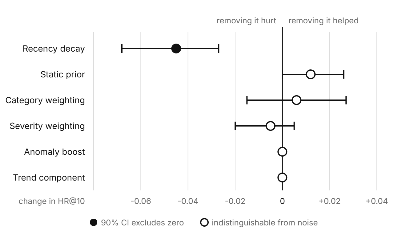
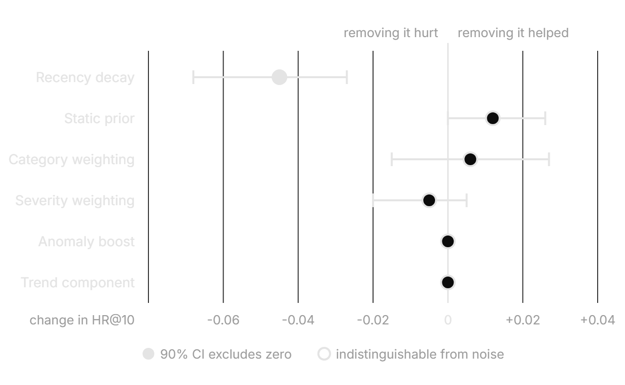
Ranked by |dHR@10|. Ablations only; the counterfactual and the floor row are discussed separately below.
| Rank | Component removed | dHR@5 | dHR@10 | dHR@10 90% CI | dPAI@10 | Distinguishable from noise? |
|---|---|---|---|---|---|---|
| 1 | recency decay | -0.071 | -0.045 | [-0.068, -0.027] | -0.135x | yes |
| 2 | static prior | +0.010 | +0.012 | [+0.000, +0.026] | +0.036x | no |
| 3 | category weighting | +0.016 | +0.006 | [-0.015, +0.027] | +0.018x | no |
| 4 | severity weighting | +0.000 | -0.005 | [-0.020, +0.005] | -0.015x | no |
| 5 | anomaly boost | +0.000 | +0.000 | [+0.000, +0.000] | +0.000x | no |
| 6 | trend component | +0.000 | +0.000 | [+0.000, +0.000] | +0.000x | no |
Reading each row
- recency decay - contributes - removing it measurably costs HR@10. What was changed: Half-life -> infinity, so 0.5^(age/hl) = 1.0: every report ever filed counts exactly as much as one filed yesterday.
- static prior - not statistically distinguishable from noise - the 90% CI on the delta, [+0.000, +0.026], contains 0. What was changed: Every locality starts from the same baseline instead of AREA_CRIME_PROFILE's low/medium/high intensity (1/3/6).
- category weighting - not statistically distinguishable from noise - the 90% CI on the delta, [-0.015, +0.027], contains 0. What was changed: murder 2.0 ... theft 1.0 all count as 1.0. This term was not in the brief's component list, but it is a real term in the score.
- severity weighting - not statistically distinguishable from noise - the 90% CI on the delta, [-0.020, +0.005], contains 0. What was changed: low/medium/high/critical (1/2/3/4) all count as 1.0.
- anomaly boost - no effect at all (exactly 0.000 on every single fold). What was changed: ANOMALY_BOOST -> 0. Expected to be a no-op: the boost sits inside
if as_of is Noneand every fold passes an as_of. - trend component - no effect at all (exactly 0.000 on every single fold). What was changed: Trend window -> 0. Expected to be a no-op: trend only shapes
predicted_score, and the backtest ranks onrisk_score.
Components that cannot affect the backtest
These are zero by construction, which is a stronger and more useful statement than "the measured effect was small". The ablation confirms it empirically (identical rankings on every fold) and the code says why:
- Anomaly boost -
predictive.pyapplies it insideif as_of is None:(line 161). Every backtest fold passes anas_ofcutoff, so the boost is never added to a graded score. The comment there is explicit and correct: live anomaly events have no historical timeline, so including them would leak present-day state into a past fold. The anomaly boost is a live-dashboard feature, not a predictive one. Nothing indocs/VALIDATION.mdis evidence for it. - Trend / forecast term -
TREND_WINDOW_DAYSproduces onlytrendandpredicted_score.compute_risksorts its output byrisk_score(line 202) andvalidation._rank_modelconsumes that order, so the forecast never reorders a single locality in a graded fold. The counterfactual below tests whether it could. - Not ablated at all, because they are monotone or cosmetic and provably cannot reorder anything: the min-max rescale to 0-100 (affine, order-preserving) and
RISK_BANDS(a label applied after ranking).
Counterfactual: does the trend term contain unused signal?
Ranking each fold by predicted_score (= risk_score x capped trend growth) instead of risk_score:
- dHR@10 = -0.005 (90% CI [-0.029, +0.019]) - not statistically distinguishable from noise - the 90% CI on the delta, [-0.029, +0.019], contains 0.
No detectable difference either way on this data. The trend term is fine to keep as a UI annotation; there is no evidence it would improve the ranking, and none that it would hurt it.
Harness self-check
With every weight flattened and decay disabled, the model's score collapses to a plain complaint count, so its ranking must equal the independently-implemented frequency baseline in validation.py. If the patches were silently not reaching the scoring path, this check would fail and every row above would be meaningless.
- PASS - stripped model HR@10 0.7420 == frequency baseline HR@10 0.7420; the patches provably reach the scoring path.
Reproduce
cd backend
PYTHONPATH=. python scripts/ablation.py --folds 8
# writes docs/ABLATION.md; uses a throwaway temp DB seeded with
# VISIONSCAN_SEED_SYNTHETIC=true, never the demo database
Deterministic within a day: the synthetic seed, the fold construction and the bootstrap seed (BOOTSTRAP_SEED = 20240601) are all fixed. The one moving part is that the synthetic window ends at seed time, so absolute levels drift slightly day to day as the window slides - the same effect documented in docs/VALIDATION.md. The paired deltas are markedly more stable than the levels, which is another reason to pair.
What this means, in plain English
The risk score is largely one idea - count the recent complaints in each locality - wearing several coats of paint. This study measures which coats are load-bearing.
- These components survive the significance test, so on this data they genuinely change which localities get patrolled: recency decay.
- static prior, category weighting point the wrong way: the model scored slightly better without them. None of those deltas clears the significance bar either, so the correct statement is "no evidence these help, and a hint they might not" - which is still a very different claim from the one the model card implies.
- Some components are purely presentational. They make the dashboard more informative and the model card more explainable, and they contribute exactly nothing to the accuracy numbers this project quotes. Anyone citing HR@10 as evidence that anomaly detection improves prediction is citing the wrong number.
- The honest summary is that a simple recency-weighted incident count does most of the work, and the elaborations around it are - on synthetic data, at 8 folds - mostly unresolvable. That is a limitation of the available evidence, not a claim that the elaborations are worthless on real data.
- The right next step is therefore not to add components. It is to get enough real folds that a delta this size becomes measurable.